1. Définition des coordonnées curvilignes
 On peut considérer qu’un point de l’espace est obtenu comme l’intersection de trois plans d’équations : \[x=cte\quad;\quad~y=cte\quad;\quad~z=cte\]
On peut dire aussi que par ce point passent des lignes de coordonnées qui sont les intersections deux à deux des plans précédents.
Effectuons alors le changement de variables suivant (supposé réversible) : \[\left\{ \begin{aligned} x=x(q_1,q_2,q_3)\\ y=y(q_1,q_2,q_3)\\ z=z(q_1,q_2,q_3) \end{aligned} \right. \qquad \left\{ \begin{aligned} q_1=q_1(x,y,z)\\ q_2=q_2(x,y,z)\\ q_3=q_3(x,y,z) \end{aligned} \right.\]
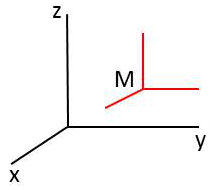
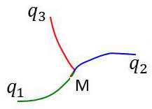 Le point \(M\) peut être alors représenté par \(M(q_1,q_2,q_3)\), c’est-à-dire qu’il se trouve à l’intersection des trois surfaces d’équations : \[q_1=cte\quad;\quad~q_2=cte\quad;\quad~q_3=cte\]
Ces surfaces sont les surfaces coordonnées. Elles se coupent deux à deux suivant 3 lignes issues de M.
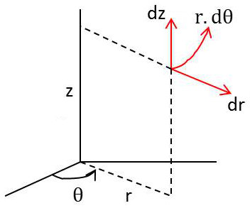
En coordonnées cylindriques :
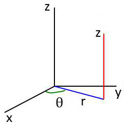 \[\left\{ \begin{aligned} &x=r~\cos(\theta)\\ &y=r~\sin(\theta)\\ &z=z \end{aligned} \right. \qquad \left\{ \begin{aligned} &q_1=r\\ &q_2=\theta\\ &q_3=z \end{aligned} \right.\]
Surfaces coordonnées en M : \[\begin{aligned} &q_1=cte\qquad\text{cylindre}~[Oz,r]\\ &q_2=cte\qquad\text{plan vertical}~[M,Oz]\\ &q_3=cte\qquad\text{plan horizontal} \end{aligned}\]
Lignes coordonnées : \[\begin{aligned} &q_3 &&\text{droite verticale} &&z~\text{varie}\\ &q_2 &&\text{cercle axe Oz} &&\theta~\text{varie}\\ &q_1 &&\text{droite horizontale} &&r~\text{varie} \end{aligned}\]
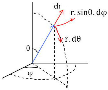
En coordonnées sphériques :
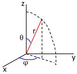 \[\left\{ \begin{aligned} &x=r~\sin(\theta)~\cos(\varphi)\\ &y=r~\sin(\theta)~\sin(\varphi)\\ &z=r~\cos(\theta) \end{aligned} \right. \qquad \left\{ \begin{aligned} q_1=r\\ q_2=\theta\\ q_3=\varphi \end{aligned} \right.\]
Surfaces coordonnées passant par M : \[\begin{aligned} &q_1=r=cte &&\text{sphère passant par M}\\ &q_2=\theta=cte &&\text{cône de sommet O et d’axe Oz}\\ &q_3=\varphi=cte &&\text{plan vertical méridien passant par M} \end{aligned}\]
Lignes coordonnées : \[\begin{aligned} &q_1~\text{varie seul} &&\text{rayon OM}\\ &q_2~\text{varie seul} &&\text{méridien}\\ &q_3~\text{varie seul} &&\text{parallèle} \end{aligned}\]
2. Élément de surface en coordonnées curvilignes (ds)²
L’élément de surface en coordonnées curvilignes est le carré de la distance de deux points.
En coordonnées cartésiennes : \[(ds)^2=(dx)^2+(dy)^2+(dz)^2\] Avec : \[dx=\frac{\partial x}{\partial q_1}~dq_1+\frac{\partial y}{\partial q_2}~dq_2+\frac{\partial z}{\partial q_3}~dq_3\]
Le \(ds^2\) est une forme quadratique homogène :
\[\begin{aligned} ds^2&=e_1^2~dq_1^2+e_2^2~dq_2^2+e_3^2~dq_3^2~+~2~e_1~e_2~dq_1~dq_2+2~e_1~e_3~dq_1~dq_3+2~e_3~e_2~dq_3~dq_2\\ e_i^2&=\Big(\frac{\partial x}{\partial q_i}\Big)^2+\Big(\frac{\partial y}{\partial q_i}\Big)^2+\Big(\frac{\partial z}{\partial q_i}\Big)^2\\ e_{ij}^2&=\frac{\partial x}{\partial q_i}~\frac{\partial x}{\partial q_j}+\frac{\partial y}{\partial q_i}~\frac{\partial y}{\partial q_j}+\frac{\partial z}{\partial q_i}~\frac{\partial z}{\partial q_j}\end{aligned}\]
En coordonnées curvilignes orthogonales : \[ds^2=e_1^2~dq_1^2+e_2^2~dq_2^2+e_3^2~dq_3^2\]
Trois expressions en découlent immédiatement : \[\begin{aligned} &\text{Élément de déplacement~:} &ds_i&=e_i~dq_i\\ &\text{Élément de surface~:} &d\sigma_{ij}&=e_i~e_j~dq_i~dq_j\\ &\text{Élément de volume~:} &d\tau&=e_1~e_2~e_3~dq_1~dq_2~dq_3 \end{aligned}\]
3. Fonctions de point en coordonnées curvilignes
3.1. Gradient
On rappelle la propriété : \[d\Phi=\overrightarrow{\rm grad}~\Phi\cdot\overrightarrow{dM}\]
On rappelle l’expression analytique : \[d\Phi=\sum_i(\overrightarrow{\rm grad}~\Phi)_i~(e_i~dq_i)\]
Et par suite : \[(\overrightarrow{\rm grad}~\Phi)_i=\frac{1}{e_i}~\frac{\partial\Phi}{\partial q_i}\]
3.2. Divergence
On applique la formule de Green-Ostrogradsky exprimant le flux sortant d’un parallélépipède élémentaire supporté par les lignes de coordonnées : \[\text{Flux}=\text{div}~\overrightarrow{V}~d\tau\qquad~d\tau=e_1~e_2~e_3~dq_1~dq_2~dq_3\]
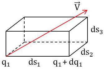 Flux entrant à gauche : \[V_1~ds_2~ds_3=e_1~e_2~V_1~dq_2~dq_3\]
Flux sortant à droite : \[V_1~e_2~e_3~dq_2~dq_3+\Big\{\frac{\partial}{\partial q_1}(e_2~e_3~V_1)~dq_1\Big\}~dq_2~dq_3\]
Flux sortant par les deux faces : \[\frac{\partial}{\partial q_1}(e_2~e_3~V_1)~dq_1~dq_2~dq_3\]
C’est-à-dire finalement : \[\text{div}\overrightarrow{V}~(e_1~e_2~e_3~dq_1~dq_2~dq_3)=\Big\{\frac{\partial}{\partial q_1}(e_2~e_3~V_1)+\frac{\partial}{\partial q_2}(e_1~e_3~V_2)+\frac{\partial}{\partial q_3}(e_1~e_2~V_3)\Big\}~dq_1~dq_2~dq_3\]
Par suite : \[\text{div}\overrightarrow{V}=\frac{1}{e_1~e_2~e_3}\sum\frac{\partial}{\partial q_1}(e_2~e_3~V_1)\]
3.3. Rotationnel
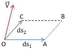 On applique la formule de Stokes élémentaire \[\{{rm circul}~\overrightarrow{V}\}_{OABC}=\{\overrightarrow{\rm rot}\overrightarrow{V}\}_3~e_1~e_2~dq_1~dq_2\]
On effectue le calcul en décomposant :
\[\begin{aligned} &\Gamma_{OA}=V_1~ds_1=e_1~V_1~dq_1\\ &\Gamma_{CB}=\Big\{e_1~V_1+\frac{\partial}{\partial q_2}(e_1~V_1)~dq_2\Big\}~dq_1\\ &\Gamma_{OC}=V_2~ds_2=e_2~V_2~dq_2\\ &\Gamma_{AB}=\Big\{e_2~V_2+\frac{\partial}{\partial q_1}(e_2~V_2)~dq_1\Big\}dq_2\end{aligned}\]
Et pour l’ensemble du circuit : \[\Gamma=\Gamma_{OA}+\Gamma_{AB}-\Gamma_{CB}-\Gamma_{OC}=\Big\{\frac{\partial}{\partial q_1}(e_2~V_2)-\frac{\partial}{\partial q_2}(e_1~V_1)\Big\}~dq_1~dq_2\]
On obtient alors : \[[\overrightarrow{\rm rot}\overrightarrow{V}]_3=\frac{1}{e_1~e_2}~\Big\{\frac{\partial}{\partial q_1}(e_2~V_2)-\frac{\partial}{\partial q_2}(e_1~V_1)\Big\}\qquad\text{et permutations}\]
Ce que l’on retient habituellement sous la forme : \[\overrightarrow{\rm rot}\overrightarrow{V}=\frac{1}{e_1~e_2~e_3} \begin{vmatrix} e_1~q_1& &e_2~q_2& &e_3~q_3\\ \\ \partial/\partial q1& &\partial/\partial q2& &\partial/\partial q3\\ \\ e_1~V_1& &e_2~V_2& &e_3~V_3 \end{vmatrix}\]
4. Évaluation de (\(e_1,~e_2,~e_3\))
 En coordonnées cylindriques [\(r,\theta,z\)]: \[\left\{ \begin{aligned} &x=r~\cos(\theta)\\ &y=r~\sin(\theta)\\ &z=z \end{aligned} \right.\]
L’expression de l’élément de surface étant : \[(ds)^2=(dr)^2+(r~d\theta)^2+(dz)^2\]
On en déduit : \[\left\{ \begin{aligned} &e_1=e_r=1\\ &e_2=e_{\theta}=r\\ &e_3=e_2=1 \end{aligned} \right.\]
Et l’expression du laplacien : \[\Delta\Phi=\frac{\partial^2\Phi}{\partial r^2}+\frac{1}{r}~\frac{\partial\Phi}{\partial r}+\frac{1}{r^2}~\frac{\partial^2\Phi}{\partial\theta^2}+\frac{\partial^2\Phi}{\partial z^2}\]
 En coordonnées sphériques [\(r,~\theta,~\varphi\)] \[(ds)^2=(dr)^2+(r~d\theta)^2+(r~\sin(\theta)~d\varphi)^2\]
On a donc : \[\left\{ \begin{aligned} &e_1=e_r=1\\ &e_2=e_{\theta}=r\\ &e_3=e_{\varphi}=r~\sin(\theta) \end{aligned} \right.\]
D’où, pour l’élément de volume : \[d\tau=r^2~\sin(\theta)~dr~d\theta~d\varphi\]
Et pour le laplacien: \[\Delta\Phi=\frac{1}{r^2~\sin^2\theta}\left\{\Big[\frac{\partial}{\partial r}\big(r^2~\sin\theta~\frac{\partial\varphi}{\partial r}\big)\Big]+\Big[\frac{\partial}{\partial\theta}\big(\sin\theta~\frac{\partial\varphi}{\partial\theta}\big)\Big]+\Big[\frac{\partial}{\partial\varphi}\big(\frac{1}{\sin\theta}~\frac{\partial\varphi}{\partial\theta}\big)\Big]\right\}\]
